Module temperature
The module temperature has a strong influence on the characteristic curve of the PV modules.
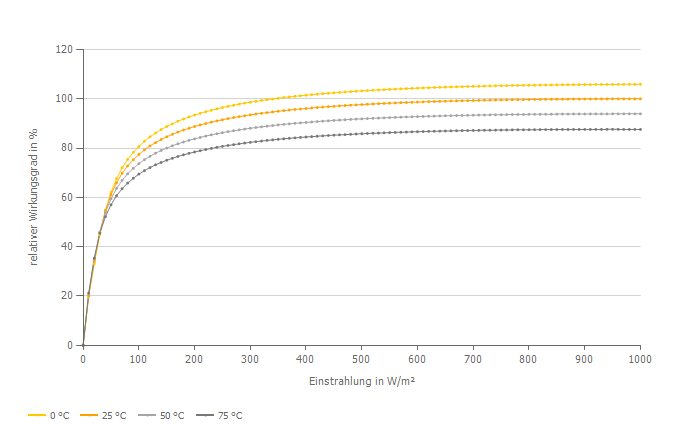
Figure 3: Typical course of module efficiency at different module temperatures.
The modules heat up depending on the installation situation, the module capacity, the type of module installation and the irradiation.
At a simulation interval of one hour, the module temperature $T_\text{Modul}$ is calculated statically from the irradiation $E$, related to the irradiation at STC ($E_\text{STC} = 1000 ~\text{W/m}^2$), and a temperature offset depending on the installation type:
$$ T_\text{Modul} = T_\text{amb} + DT \cdot \frac{E}{E_\text{STC}} $$
Table 1: Heating DT in relation to the outside temperature, e.g. at irradiation $E = 1000 ~\text{W/m}^2$
| DT | Installation situation |
|---|---|
| 29 K | roof-parallel, well ventilated |
| 32 K | roof-integrated – rear-ventilated |
| 43 K | roof-integrated – not ventilated |
| 28 K | mounted – roof |
| 22 K | mounted – free area |
| 20 K | mounted – Floating PV |
Source: DGS-Leitfaden Photovoltaische Anlagen, 3. Auflage, also Marco Rosa-Clot, Giuseppe Marco Tina, ‘Floating PV plants’ Academic Press, 2020.
The static temperature model is unsuitable for a simulation in minute time steps with alternating irradiation, since it does not take the thermal inertia of the module into account. A dynamic temperature model is therefore used for a simulation interval of one minute. The module is represented by a capacity $C$ with the module temperature $T_\text{ Modul}$:
$$ \frac{dQ}{dt} = C \cdot \frac{dT_\text{Modul}}{dt} $$
A specific heat capacity of $830\frac{\text{J}}{\text{kg K}}$ and a module mass according to the module data set is used to calculate the heat capacity $C$.
The module is heated by the irradiation. This is contrasted by heat losses:
$$ \frac{dQ_\text{Verluste}}{dt} = UA \cdot \left( T_\text{Modul} - T_\text{Amb} \right) $$
The heat loss rate $UA$ is determined from the static temperature offset
$$ UA = \frac{E_\text{STC}}{DT} $$
See also