PV field
The equivalent circuit diagram
In a PV system, several PV modules are interconnected to form a PV field. The modules can be connected in series to form module strings. If several of these strings are connected in parallel, the PV field is obtained. The picture below illustrates the wiring in a sketch.
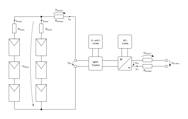
Equivalent circuit diagram of PV modules, string, DC and AC cabling (resistors)
Both the individual strings and the DC and AC lines are afflicted with ohmic resistances. From the electrical circuit diagram the following results for the DC side:
-
The currents through the modules of a string are always the same, while the voltage in the string can be understood as the sum of the module voltages. In addition, there is the voltage drop across the resistance of the string lines.
$I_\text{Strang} = I_\text{Modul 1} = I_\text{Modul 2} = …$
$U_\text{Strang} = U_\text{Modul 1} + U_\text{Modul 2} + … -U_\text{Drop, Strang}$ -
The voltages of two parallel strings are always the same, while the currents can be different. In total, the string currents result in the DC current. The DC voltage is the sum of the string voltage and the voltage drop across the line resistance.
$U_\text{Strang} = U_\text{Strang 1} = U_\text{Strang 2}$
$I_\text{DC} = I_\text{Strang 1} + I_\text{Strang 2}$
$U_\text{DC} = U_\text{Strang} + U_\text{Drop, DC}$
For the AC side, between the inverter and the grid, this results in:
-
The AC power on the inverter side results from the DC power ($U_\text{DC}\cdot I_\text{DC}$) and the efficiency of the inverter. The efficiency depends on the DC power and the DC voltage
$P_\text{AC} = \eta_\text{U(DC),P(DC)} \cdot U_\text{DC} \cdot I_\text {DC}$ -
The AC voltage on the inverter side depends on the mains voltage, the AC current and the resistance of the AC cables.
$U_\text{AC}=U_\text{AC,Netz} + I_\text{AC}\cdot R_\text{AC}$
Characteristic superposition
In the simulation, the DC-side characteristic curve of the PV field is calculated as follows: First, the V-C curve is calculated for each PV module. The module characteristics are superimposed for each string together with the string resistance to form a string characteristic.
Example: Characteristic curve superimposition for string 1, consisting of two modules which have different V-C characteristics due to shading
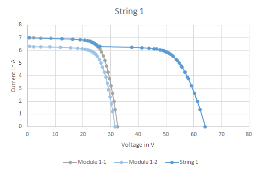
The characteristic curves of two modules in string 1 are superimposed to the string characteristic curve. The currents remain the same, the voltages add up.
Example: Characteristic curve overlay for string 2, also consisting of two modules which have different V-C characteristics due to shading
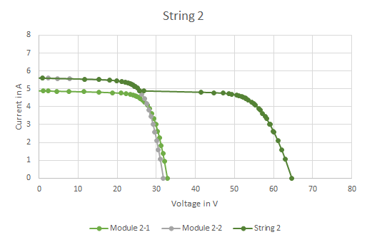
The characteristic curves of two modules in string 2 are superimposed to form a second string characteristic curve. The currents remain the same, the voltages add up.
Once the string characteristics have been created, they are superimposed on the field characteristic:
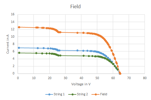
The field characteristic is superimposed from the two string characteristics. This time the voltages remain the same, while the currents add up.
In this way, the field characteristic curve of the PV system is obtained at any time during the simulation. If the system has several sub-surfaces, the process is repeated for each of these sub-surfaces. The field characteristic is now transferred to the MPP tracker of the inverter connected to the PV field. This searches the characteristic curve for the point of maximum power. In this example, a maximum field power of 530 W would result at about 51 V DC voltage. The DC current is therefore approx. 10,4 A .
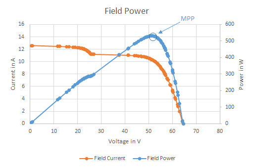
The current-voltage characteristic results in the power-voltage characteristic. The point of maximum power is called MPP (maximum power point).
AC conversion, checking for current, voltage and power limits
Please note that the MPP Tracker can only search within its own current and voltage limits on the field characteristic. It can therefore happen that the true point of maximum performance lies outside the tracking range of the MPP tracker.
In this example, this results in $U_\text{DC}=51,\text{V}$, $I_\text{DC}=10.4,\text{A}$ and $P_\text{DC}=530,\text{W}$. In the inverter, the AC power is now calculated according to the efficiency characteristic curve. The efficiency curve depends on the DC voltage (more precisely: …the deviation of the DC voltage from the nominal voltage of the MPP tracker) and the DC power.
The AC voltage and AC current then result from the AC power, the mains voltage and the AC line resistance. Here, too, the resulting power, voltage or current can exceed the inverter’s limits. If this is the case, the limits are again reported to the MPP tracker, which with these restrictions searches again for the point of maximum power on the field characteristic.
In this example we say that the maximum AC power of the inverter is 500 W. The operating point determined by the MPP tracker is now higher at 530 W. Therefore, the MPP tracker must now determine a new operating point that does not exceed 500 W. In order to keep the ohmic losses as small as possible, the search is always made in the direction of higher voltages. In this case, the first operating point not exceeding 500 W would be about 55 V and 8.9 A.
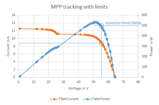
The current-voltage characteristic results in the power-voltage characteristic. The point of maximum power is called MPP (maximum power point).
Calculation of losses in the PV field
If the point of maximum power is found, the PV field is informed which operating point on the field curve the MPP tracker has selected – in this example about $U_\text{DC}=55,\text{V}$ and $I_\text{DC}=8.9,\text{A}$, since otherwise the power limits would have been exceeded on the AC side.
These values now result in the ohmic losses at the DC and string resistors.
Everything else, i.e. the actual string voltage and the currents through the modules, also result from the selected operating point:
$P_\text{Verlust,DC}=I_\text{DC}^2 \cdot R_\text{DC}$
$U_\text{Drop,DC}=I_\text{DC} \cdot R_\text{DC}$
$U_\text{Strang}=U_\text{DC} - U_\text{Drop,DC}$
See also