Characteristic curve models
To describe the characteristic curve of a solar cell, a model is used whose task it is to represent the electrical or thermal behavior of the cell over as wide a range of external influences as possible.
Basically, the models can be divided into empirical and physically oriented models. Empirical models are based on measurement results from real photovoltaic modules or cells, from which parameters for fit functions are usually obtained. These models can achieve very high imaging accuracy for the measured modules, while, as expected, they function worse with non-measured modules, since no parameters were determined here.
Physical models attempt to present the real processes in photovoltaic semiconductors in a generally valid manner. This means that they can also be applied with some accuracy to modules measured only minimally (by the manufacturer). However, the physical models also require some parameters, which must either also be determined empirically or are included in the modeling in the form of standard values. The most common physical models are the one- and two-diode model.
In PV*SOL® either the PV*SOL® model or the two-diode model is used to calculate the characteristic curves.
PV*SOL® model
Basics
It is primarily a mathematical model, but in addition to the electrical data provided by the manufacturer, it requires a further set of electrical data as unconditional input variables at a weak light point near $20,%$ of the STC irradiation. The characteristic curve of the filling factor as a function of the irradiation is used. Since the short-circuit current is largely linear from the irradiance, the fill factor function can be used to derive the variables in the MPP. Once these values have been calculated, the interpolation between the three points is exponential. Thus the model of PV*SOL® allows the direct calculation of both the key parameters and the characteristic of a module with given irradiation.
The low light operating point
If the additionally required information about the low light point is not given – ideally these are provided by the module manufacturers – standard values are calculated depending on the module technology.
For this purpose, some parameters are determined first. Irradiation at the low light operating point $E_\text{SL}$ determines where the fill factor assumes the (maximum) value $ff_\text{Extra} \cdot FF_\text{STC}$. Parameters $E_\text{min}$ and $k$ serve for iterative determination of other parameters.
First the fill factor in the low light point $FF_\text{SL}$ is calculated:
$$ FF_\text{SL} = ff_\text{Extra} \cdot FF_\text{STC} \qquad\qquad (1)$$
The open circuit voltage at the low light operating point $U_\text{OC,SL}$ is determined by
$$ U_\text{OC,SL} = U_\text{OC,STC} \cdot \frac{\log{ \left( \frac{E_\text{SL}}{E_\text{min}}\right)}}{\log{ \left( \frac{E_\text{STC}}{E_\text{min}}\right)}} \qquad\qquad (2)$$
Table 2: Default values of the PV*SOL® model for different module technologies
| Module technology | $E_\text{SL}$ | $E_\text{min}$ | $k$ | $ff_\text{Extra}$ |
|---|---|---|---|---|
| Amorphous Si | $150$ | $2.2\cdot 10^{-6}$ | $0.9685$ | $1.03$ |
| CdTe | $200$ | $1.0\cdot 10^{-7}$ | $1.0000$ | $1.03$ |
| Amorph | $250$ | $5.0\cdot 10^{-8}$ | $1.0300$ | $1.00$ |
| CIS | $300$ | $0.1$ | $1,0000$ | $1.10$ |
| HIT | $200$ | $1.0\cdot 10^{-7}$ | $1.0400$ | $1.04$ |
| All others | $300$ | $0.1$ | $1.0000$ | $1.05$ |
The smaller $E_\text{min}$ and the larger $E_\text{SL}$ are selected, the smaller the decrease of the open circuit voltage at the low light operating point will be (see example in Figure 4 with $U_\text{OC,STC}=0.6,\text{V}$).
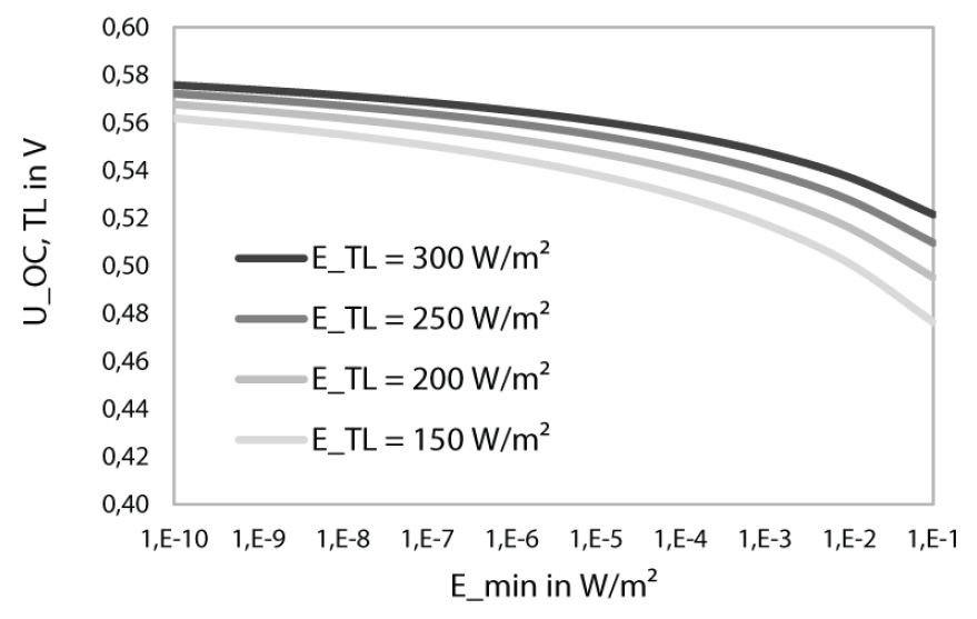
Figure 4: The low light open-circuit voltage as a function of $E\_\text{min}$ and $E\_\text{SL}$.
As mentioned above, the short-circuit current is linearly reduced according to
$$ I_\text{SC,TL} = I_\text{SC,STC} \frac{E_\text{TL}}{E_\text{STC}} \qquad\qquad (3)$$
The current and voltage in the MPP are first set to $U_\text{MPP,SL} = 1.1\cdot U_\text{OC,SL}$ and $I_\text{MPP,SL}=0$. Then the equations for the current
$$ I_\text{MPP,SL}=k\cdot I_\text{SC,SL} \frac{I_\text{MPP,STC}}{I_\text{SC,STC}} \qquad\qquad (4)$$
and the voltage
$$ U_\text{MPP,SL} = FF_\text{SL} \cdot U_\text{OC,SL} \frac{I_\text{SC,STC}}{I_\text{MPP,STC}} \qquad\qquad (5)$$
in the MPP, and the correction of the factor $k$ with
$$ k = 1,1 \frac{U_\text{MPP,SL}}{U_\text{OC,SL}} \qquad\qquad (6)$$
repeated until $U_\text{MPP,SL}\gt U_\text{OC,SL}$ or $k\gt 2$. Once the low light quantities have been determined, they can be calculated for each irradiation and temperature.
Fill factor
The characteristic behavior of the fill factor $FF$ is now represented by the inverse of a quadratic equation, where $E$ corresponds to the global radiation on module level:
$$ FF=\frac{E}{a\cdot E^{2} + b\cdot E + c} \qquad\qquad (7)$$
The coefficients $a$, $b$ and $c$ are calculated depending on the size of the low light fill factor as follows:
$$ a = \begin{cases} 0 &\text{wenn } FF_\text{SL} = FF_\text{STC}\cr \frac{E_\text{ STC} \left( FF_\text{ SL}-FF_\text{ STC} \right) }{FF_\text{ SL}\cdot FF_\text{ STC}\cdot \left( E_\text{ SL}-E_\text{ STC} \right) ^2} &\text{wenn } FF_\text{ SL}\gt FF_\text{ STC}\cr \frac{E_\text{ SL} \left( FF_\text{ STC}-FF_\text{ SL} \right)}{FF_\text{ STC}\cdot FF_\text{ SL}\cdot \left( E_\text{ STC}-E_\text{ SL} \right) ^2} &\text{wenn } FF_\text{ SL}\lt FF_\text{ STC}\cr \end{cases} \qquad\qquad (8) $$
$$ b = \begin{cases} \frac{1}{FF_\text{SL}} &\text{wenn } FF_\text{SL} = FF_\text{STC}\cr \frac{1-2a \cdot E_\text{SL}FF_\text{SL}}{FF_\text{SL}} &\text{wenn } FF_\text{SL} \neq FF_\text{STC}\cr \end{cases} \qquad\qquad (9) $$
$$ c = \begin{cases} 0 &\text{wenn } FF_\text{SL} = FF_\text{STC}\cr a \cdot E_\text{SL}^{2} &\text{wenn } FF_\text{SL} \gt FF_\text{STC}\cr a \cdot E_\text{STC}^{2} &\text{wenn } FF_\text{SL} \lt FF_\text{STC}\cr \end{cases} \qquad\qquad (10) $$
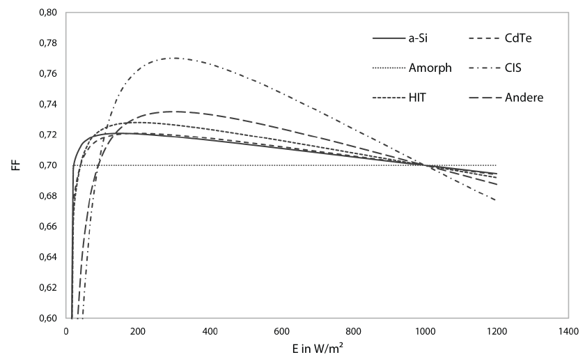
Figure 5: The fill factor above the irradiation for different module technologies.
For illustration, figure 5 shows the different fill factor curves as a function of irradiance. A fictitious fill factor of 0.7 was assumed for all technologies under STC conditions.
Idle
Analogous to the calculation at the low light point according to equation (2-1-2), the open circuit voltage $ U_\text{OC} $ is now calculated with
$$ U_\text{OC} = U_\text{OC,STC} \cdot \frac{\ln\left(\frac{E}{G_0}\right)}{\ln\left(\frac{E_\text{STC}}{G_0}\right)} + \alpha_\text{U} \left(T_\text{M}-T_\text{STC}\right) \qquad\qquad (11)$$
whereby it should be noted that the temperature coefficient of the voltage $\alpha_\text{U}$ must be used here in $\frac{\text{V}}{\text{K}}$. The auxiliary quantity $G_0$ ensures that the open circuit voltage at partial load is $U_\text{OC,SL}$:
$$ G_0 = \exp\left( \frac{U_\text{OC,STC}\ln(E_\text{SL}) - U_\text{OC,SL}\ln(E_\text{STC})}{U_\text{OC,STC} - U_\text{OC,SL}} \right)\qquad\qquad (12)$$
Short-circuit current
The short-circuit current $C_\text{SC}$ is now calculated depending on whether the current irradiance $E$ is smaller or larger than the irradiance at the low light operating point $E_\text{SL}$. If it is lower, the quadratic relationship
$$ I_\text{SC} = d \cdot E^2 + \left( e + \frac{\Delta I_\text{SC}}{E_\text{STC}} \right) E \qquad\qquad (13)$$
with
$$ d = \frac{I_\text{SC,STC} - \left( \frac{I_\text{SC,STC}-I_\text{SC,SL}}{E_\text{STC}-E_\text{SL}} \right) E_\text{STC}}{E_\text{SL}^2} \qquad\qquad (14)$$
and
$$ e = \frac{I_\text{SC,STC} - I_\text{SC,SL}}{E_\text{STC}-E_\text{SL}} + 2 \frac{I_\text{SC,STC} - \left( \frac{I_\text{SC,STC}-I_\text{SC,SL}}{E_\text{STC}-E_\text{SL}} \right) E_\text{STC}}{E_\text{SL}} \qquad\qquad (15)$$
applies. The temperature dependence is included in the calculation via
$$ \Delta I_\text{SC} = \alpha_\text{I,SC} \left( T_\text{M} - T_\text{STC} \right) \qquad\qquad (16)$$
(the absolute value must also be used here, so $[\alpha_\text{I}] = \frac{\text{A}}{\text{K}}$). If the irradiation is greater than that of the weak-light point, there is a linear relationship between short-circuit current and irradiation, which is the same for all models.:
$$ I_\text{SC} = I_\text{SC,STC} - \left( \frac{I_\text{SC,STC} - I_\text{SC,SL}}{E_\text{STC} - E_\text{SL}} \right) E_\text{STC} + \left( \frac{I_\text{SC,STC} - I_\text{SC,SL}}{E_\text{STC} - E_\text{SL}} + \frac{\Delta I_\text{SC}}{E_\text{STC}} \right) E \qquad\qquad (17)$$
MPP
The calculation of the MPP current is also divided into two ranges – according to the calculation of the short-circuit current. In the range of irradiation between $0$ and the low light point, the following rule applies
$$ I_\text{MPP} = I_\text{SC} \cdot \upsilon_\text{I} \cdot \sqrt{\zeta_\text{P}} \qquad\qquad (18)$$
with
$$ \upsilon_\text{I} = b\upsilon_\text{I} + m\upsilon_\text{I} \cdot E \cdot \sqrt{\zeta_\text{P}} \qquad\qquad (19)$$
$$ b\upsilon_\text{I} = \frac{I_\text{MPP,STC}}{I_\text{SC,STC}} - \left( \frac{ \frac{I_\text{MPP,STC}}{I_\text{SC,STC}} - \frac{I_\text{MPP,SL}}{I_\text{SC,SL}} }{E_\text{STC} - E_\text{SL}} \cdot E_\text{STC} \right) \qquad\qquad (20)$$
$$ m\upsilon_\text{I} = \frac{ \frac{ I_\text{MPP,STC}}{I_\text{SC,STC}} - \frac{I_\text{MPP,SL}}{I_\text{SC,SL} }}{ E_\text{STC} - E_\text{SL} }\qquad\qquad (21)$$
and the temperature coefficient of the power $\alpha_\text{P}$ (this time between $0$ and $1$)
$$ \zeta_\text{P} = \frac{ ( 1+\alpha_\text{P} (T_\text{M}-T_\text{STC} ))(U_\text{OC,STC} I_\text{SC,STC}) }{ (U_\text{OC,STC} + \Delta U_\text{OC}) (I_\text{SC,STC} + \Delta I_\text{SC}) } \qquad\qquad (22)$$
Analogous to the current $\Delta U_\text{OC}$ is calculated:
$$ \Delta U_\text{OC} = \alpha_\text{U} (T_\text{M}-T_\text{STC}) \qquad\qquad (23)$$
If the irradiation is above the low light point, the MPP current is simply scaled with the ratio of MPP and short-circuit current under STC conditions and you get
$$ I_\text{MPP} = \frac{I_\text{MPP,STC}}{I_\text{SC,STC}} \cdot I_\text{SC} \qquad\qquad (24)$$
This calculates the three key points short-circuit, open circuit and MPP.
Characteristic curve
Between these points the characteristic can be interpolated exponentially. In the range between short circuit and MPP the following applies
$$ I_1(U) = bv + mv \cdot \exp(U\cdot kv) - \frac{I_\text{SC} - I_\text{MPP}}{2 U_\text{MPP}} \cdot U \qquad\qquad (25)$$
with
$$ bv = \frac{ I_\text{SC}\cdot\exp(kv\cdot U_\text{MPP}) - \left( I_\text{MPP} + \frac{I_\text{SC} - I_\text{MPP}}{2} \right) }{ \exp(kv\cdot U_\text{MPP})-1 } \qquad\qquad (26)$$
$$ mv = \frac{ I_\text{MPP}-I_\text{SC}+\frac{I_\text{SC}-I_\text{MPP}}{2} }{ \exp(kv\cdot U_\text{MPP})-1 } \qquad\qquad (27)$$
$$ kv = \frac{\text{invers}(y)}{U_\text{MPP}} \qquad\qquad (28)$$
$$ y = \left( \frac{I_\text{MPP} + \frac{I_\text{SC}-I_\text{MPP}}{2} }{ I_\text{SC} - I_\text{MPP} + \frac{I_\text{SC}-I_\text{MPP}}{2} } \right) \qquad\qquad (29)$$
The function $\text{invers}(y)$ returns an approximation of the $x$ value for a known $y$ of the function
$$ y = \frac{x}{\exp(x-1)} \qquad\qquad (30)$$
since this is not explicitly calculable.
In the second range – between MPP and open circuit – the characteristic is approximated as follows:
$$ I_2(U) = bn + mn \exp(U\cdot kn) - \frac{I_\text{SC} - I_\text{MPP}}{2U_\text{MPP}} (U-U_\text{OC}) \qquad\qquad (31)$$
with
$$ bn = \frac{I_\text{MPP}-I_\text{rd}}{1-\exp(kn(U_\text{MPP}-U_\text{OC}))} \qquad\qquad (32)$$
$$ mn = \frac{ -I_\text{MPP}+I_\text{rd} }{ \exp(kn\cdot U_\text{OC}) - \exp(kn\cdot U_\text{MPP}) } \qquad\qquad (33)$$
$$ kn = \frac{ \text{invers}(y) }{U_\text{OC} - U_\text{MPP}} \qquad\qquad (34)$$
$$ y = \frac{ U_\text{OC} }{U_\text{MPP}} - 1 \qquad\qquad (35)$$
$$ I_\text{rd} = \frac{ I_\text{SC}-I_\text{MPP} }{ 2\cdot U_\text{MPP} } (U_\text{OC} - U_\text{MPP}) \qquad\qquad (36)$$
One-diode model
Basics
If the equivalent circuit diagram of a PV cell consisting of a power source with a diode connected in parallel is extended by a parallel ($R_\text{P}$) and a series resistor ($R_\text{S}$), the circuit diagram of the single diode model is obtained:
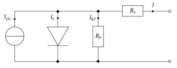
Figure 6: Equivalent circuit diagram of the single diode model.
The current source models the generation of electron-hole pairs, which are separated by the voltage in the p-n junction and then derived via an external load. The p-n junction itself is represented in the circuit diagram by the diode. Recombinations of the electron-hole pairs, as they occur, for example, at the edge of the cell, are taken into account by the parallel resistance, while the series resistance reflects the losses caused by contacts, lines and the like.
Thus, the current that can be taken from the cell at a given voltage at the terminals can be formulated as an extension of the Shockley equation as follows:
$$ I = I_\text{ph} - I_\text{S} \cdot \left( \exp\left( \frac{U+IR_\text{s}}{m\cdot U_\text{T}} \right)-1 \right) - \frac{U+IR_\text{s}}{R_\text{p}} \qquad\qquad (37)$$
The photocurrent $I_\text{ph}$ is therefore always slightly above the current to be measured, i.e. at STC conditions slightly above the short circuit current $I_\text{SC,STC}$. It is linearly dependent on the irradiation $E$ and increases with increasing cell temperature $T$:
$$ I_\text{ph} = (C_1+C_2\cdot T)E \qquad\qquad (38)$$
The parameters $C_1$ and $C_2$ are cell- or module-dependent, but can be easily calculated from the manufacturer’s specifications at least approximately.
The saturation current $I_\text{S}$ can be described in more detail with
$$ I_\text{S} = C_\text{S} T^{\kappa} \exp\left( -\frac{E_\text{Gap}}{m\text{k}T} \right) \qquad\qquad (39)$$
and is usually in the order of $10^{-11}…10^{-9}\text{A}$. The material- and technology-dependent constant $C_\text{S}$ has values around $10^{2}\frac{\text{A}}{\text{K}^3}$, the exponent of temperature $\kappa$ in the literature is usually specified as $3$, $E_\text{Gap}$ is the band gap of the cell material (z.B. $E_\text{Gap,Si}(T=300\text{K})\approx 1,12\text{eV}$ of silicon at room temperature). The temperature or thermoelectric voltage $U_\text{T}$ is calculated with
$$ U_\text{T} = \frac{\text{k}T}{e} \qquad\qquad (40)$$
Sometimes the diode factor $m$ is still included in the calculation. Ultimately, however, it is of course equivalent to consider the diode factor separately and not as part of the thermoelectric voltage. Physically, the diode factor should represent recombination effects, e. g. in the p-n transition.In the literature, $m=1$ is set in most cases, although it is doubtful that all cell technologies exhibit similar recombination behavior.
Finally, the serial resistance $R_\text{s}$ and the parallel resistance $R_\text{p}$ remain for the description of the formula characters used in equation $(37)$. For modern solar cells the resistances should be in the range $R_\text{s}=10^{-1}\Omega$ or $R_\text{p}=10^2\Omega$.
The series resistance can be assumed to be largely independent of irradiation and temperature, while the parallel resistance of the irradiation is inversely proportional to $E$.
$$ R_\text{p}(E) = R_\text{p,STC}\frac{E_\text{STC}}{E} \qquad\qquad (41)$$
Boundary conditions
In general, under STC conditions from the characteristic equation $(37)$, the four situations defined by the data sheet data can be described as follows. At no load, the voltage assumes the value of the no load voltage $U_\text{OC,STC}$ specified on the data sheet, the current is $0$:
$$ 0 = I_\text{ph}-I_\text{S}\cdot\left( \exp\left( \frac{U_\text{OC,STC}}{mU\text{T}} \right)-1 \right) - \frac{U_\text{OC,STC}}{R_\text{p}} \qquad\qquad (42)$$
In the short-circuit, the voltage $0$ is again used, while the current takes on the data sheet value:
$$ I_\text{SC,STC} = I_\text{ph}-I_\text{S} \cdot \left( \exp\left( \frac{I_\text{SC,STC} \cdot R_\text{s}}{m \cdot U_\text{T}} \right)-1 \right)-\frac{I_\text{SC,STC} \cdot R_\text{s}}{R_\text{p}} \qquad\qquad (43)$$
At point of maximum power (MPP), currents and voltages are also given:
$$ I_\text{MPP,STC} = I_\text{ph}-I_\text{S}\left( \exp\left( \frac{U_\text{MPP,STC}+I_\text{MPP,STC}\cdot R_\text{s}}{m\cdot U_\text{T}} \right)-1 \right)-\frac{U_\text{MPP,STC}+I_\text{SC,STC}\cdot R_\text{s}}{R_\text{p}} \qquad\qquad (44)$$
Furthermore, the power gradient in the MPP must be $0$. So:
$$ \frac{dP}{dU}(U=U_\text{MPP,STC})\stackrel{!}{=}0 $$
$$ I_\text{ph}-C_\text{S}T^3\exp\left( -\frac{E_\text{Gap}}{m\text{k}T} \right) \cdot \left( \exp\left( \frac{U_\text{MPP,STC} + I_\text{MPP,STC} \cdot R_\text{S}}{m\cdot U_\text{T}} \right) -1 \right)-\frac{U_\text{MPP,STC}+I_\text{SC,STC}\cdot R_\text{S}}{R_\text{P}} $$ $$+ U_\text{MPP,STC}\cdot\left(-\frac{C_\text{S}T^{2}}{m\cdot U_\text{T}}\cdot\exp\left(-\frac{E_\text{Gap}}{mkT}\right)\cdot\left(\frac{U_\text{MPP,STC} + I_\text{MPP,STC} \cdot R_\text{S}}{m\cdot U_\text{T}}\right)-\frac{1}{R_\text{P}}\right)\stackrel{!}{=} 0 \qquad (45) $$
Dynamics
In order to be able to estimate how the one-diode model reacts to the various parameters, C-V characteristics are shown below, in each of which one parameter is varied. Unless otherwise stated in the diagram, the parameters are defined as follows:
$$I_\text{ph}=3,17,\text{A} \qquad T=300,\text{K} \qquad E_\text{Gap}=1,107,\text{eV}$$ $$m=1 \qquad R_\text{s}=0,01,\Omega \qquad R_\text{p}=100,\Omega \qquad C_\text{S}=300,\frac{\text{A}}{\text{K}^3}$$
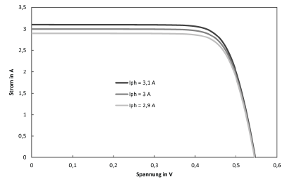
Figure 7: Variation of the photocurrent.
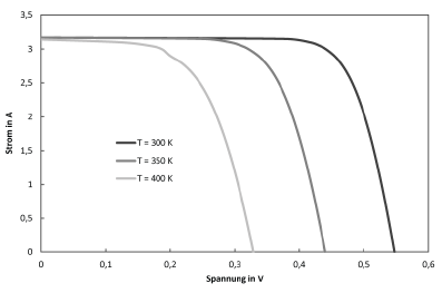
Figure 8: Variation of temperature.
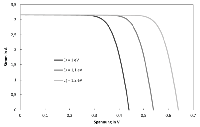
Figure 9: Variation of the gap.
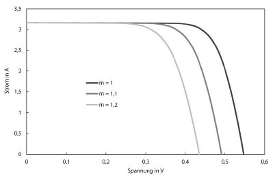
Figure 10: Variation of the diode factor.
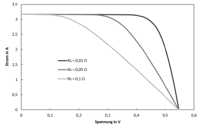
Figure 11: Variation of the series resistance.
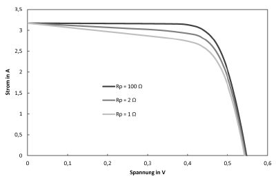
Figure 12: Variation of the parallel resistance.
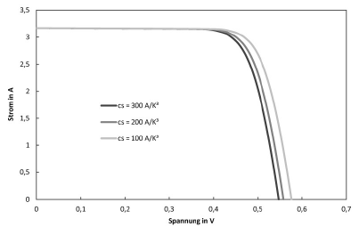
Figure 13: Variation of the saturation factor.
Parameter determination
Normally, only the basic electrical data under STC conditions of the module can be taken from the data sheets of the PV module manufacturers. These include the open circuit voltage $V_\text{OC,STC}$, the short circuit current $C_\text{SC,STC}$, voltage and current in the MPP $V_\text{MPP,STC}$ and $C_\text{MPP,STC}$, and in most cases the temperature coefficients of the open circuit voltage $\alpha_\text{U}.
The parameters of the one-diode model can be calculated from these data.
Two-diode model
Basics
The two-diode model adds another diode parallel to the first to the single-diode model described above, which generally contributes to an improvement in imaging accuracy in the MPP range.
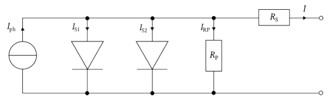
Figure 14: Equivalent circuit diagram of the two-diode model.
A further term is added to the mathematical model for the characteristic curve accordingly. The diode factors $m_1$ and $m_2$ are usually set to 1 and 2 respectively, and the saturation currents $I_\text{S1}$ and $I_\text{S2}$ also differ in amount.
$$ I=I_\text{ph} - I_\text{S1} \cdot \exp\left(\frac{U+I\cdot R_\text{S}}{m_1\cdot U_\text{T}}\right) - I_\text{S2}\cdot\exp\left( \frac{U+I\cdot R_\text{S}}{m_2\cdot U_\text{T}} \right) - \frac{U+I\cdot R_\text{S}}{R_\text{P}} \qquad\qquad (46)$$
The photocurrent $C_\text{ph}$ is calculated analogous to the one-diode model according to equation (38). The saturation currents are calculated via
$$ I_\text{S1}=C_\text{S1}\cdot T^{\kappa_1} \cdot \exp\left( -\frac{E_\text{Gap}}{m_1\cdot k \cdot T} \right) \qquad\qquad (47)$$
and
$$ I_\text{S2}=C_\text{S2}\cdot T^{\kappa_2} \cdot \exp\left( -\frac{E_\text{Gap}}{m_2\cdot k \cdot T} \right) \qquad\qquad (48)$$
The exponents $\kappa_1$ and $\kappa_2$ are almost unanimously specified in the literature as $3$ and $\frac{5}{2}$. Thus, the two-diode model contains two parameters more than the single-diode model: the diode factor $m_2$ and the saturation factor $C_\text{S2}$. Furthermore, there are approaches that question the exact value of exponents of temperatures $\kappa_1$ and $\kappa_2$ in the equations for the saturation currents and arrive at values deviating from $3$ and $\frac{5}{2}$.
Boundary conditions
Analogous to the single diode model, the four boundary conditions can be set up. The open circuit equation
$$ 0=I_\text{ph}-I_\text{S1}\cdot \left( \exp\left( \frac{U_\text{OC,STC}}{m_1 \cdot U_\text{T}} \right)-1 \right) - I_\text{S2}\cdot\left(\exp\left( \frac{U_\text{OC,STC}}{m_2\cdot U_\text{T}} \right)-1 \right)-\frac{U_\text{OC,STC}}{R_\text{P}} \qquad\qquad (49)$$
the short-circuit equation
$$ I_\text{SC,STC}=I_\text{ph}-I_\text{S1}\cdot \exp\left( \frac{I_\text{SC,STC}\cdot R_\text{S}}{m_1\cdot U_\text{T}} \right)-I_\text{S2}\cdot \exp\left( \frac{I_\text{SC,STC}\cdot R_\text{S}}{m_2\cdot U_\text{T}} \right)-\frac{I_\text{SC,STC}\cdot R_\text{S}}{R_\text{P}} \qquad\qquad (50)$$
and the two equations for the MPP
$$ I_\text{MPP,STC} = I_\text{ph} - I_\text{S1}\cdot \exp\left( \frac{U_\text{MPP,STC} + I_\text{MPP,STC}\cdot R_\text{S}}{m_1\cdot U_\text{T}} \right) $$ $$ -I_\text{S2}\cdot\exp\left( \frac{U_\text{MPP,STC} + I_\text{MPP,STC}\cdot R_\text{S}}{m_2\cdot U_\text{T}} \right) - \frac{U_\text{MPP,STC} + I_\text{MPP,STC}\cdot R_\text{S}}{R_\text{P}} \qquad\qquad (51)$$
and
$$ \frac{dP}{dU}\left(U=U_\text{MPP,STC}\right)\stackrel{!}{=}0 $$
$$ I_\text{ph}-I_\text{S1}\cdot \exp\left( \frac{U_\text{MPP,STC} + I_\text{MPP,STC} \cdot R_\text{S}}{m_1\cdot U_\text{T}} \right) - I_\text{S2}\cdot \exp\left(\frac{U_\text{MPP,STC} + I_\text{MPP,STC} \cdot R_\text{S}}{m_2\cdot U_\text{T}} \right) $$ $$- \frac{U_\text{MPP,STC} + I_\text{MPP,STC} \cdot R_\text{S}}{R_\text{P}} $$ $$ +U_\text{MPP,STC}\cdot\left( -\frac{e\cdot C_\text{S1}T^2}{m_1\cdot k}\cdot\exp\left( \frac{U_\text{MPP,STC} + I_\text{MPP,STC}\cdot R_\text{S}}{m_1\cdot U_\text{T}} \right) -\frac{e\cdot C_\text{S2}\cdot T^{\frac{3}{2}}}{m_2\cdot k} \exp\left( \frac{U_\text{MPP,STC} + I_\text{MPP,STC}\cdot R_\text{S}}{m_2\cdot U_\text{T}}\right)-\frac{1}{R_\text{P}}\right)\stackrel{!}{=}0 \qquad (52)$$
Dynamics
Essentially, the C-V characteristic of the two diode model behaves similarly to the one-diode model when the parameters are varied. For the sake of completeness, here are the variations of the two new parameters:
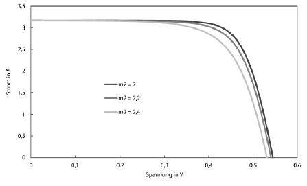
Figure 15: Variation of the second diode factor.
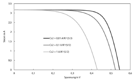
Figure 16: Variation of the second saturation factor.
It can be seen that the characteristic reacts less sensitively to the variation of the second diode factor than to that of the first. The reason for this is on the one hand that the second diode factor is smaller by orders of magnitude than the first ($C_\text{S2} \approx 10^{-2} ~\text{A} \cdot \text{K}^{-\frac{5}{2}}$), on the other hand the temperature in this term is potentiated less.
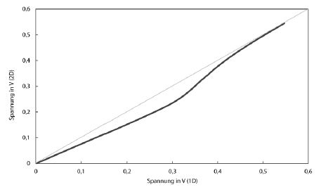
Figure 17: Influence of the second diode term in comparison to the first.
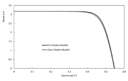
Figure 18: Both models side by side.
Figure 17 shows exactly how the second term affects the characteristic curve. The voltage calculated with the two-diode model was applied over the voltage calculated with the single-diode model. It should be noted that the second diode term has the most concise effect in the area below the MPP voltage. In the short-circuit and open circuit points, however, the two-diode model does not deliver any deviating results. Figure 18 shows the C-V characteristics of both models together.
Parameter determination
In the two-diode model, the second diode term adds two more parameters to those already to be determined in the single-diode model.
- The second saturation factor $C_\text{S2}$ and
- the second diode factor $m_2$
So you get a system with at first eight unknowns. Since the band gap $E_\text{Gap}$ and the diode factors $m_1$ and $m_2$ cannot be calculated explicitly in this case, they are replaced by the values commonly used in the literature.
Under these conditions it is possible to calculate the parameters for the two diode model from data sheet data.
See also